Computational Physics (Part2)【未完结】

Computational Physics (Part2)

[TOC]

5. Roots and Extermal Points

5.1 Root Finding

If there is exactly one root in the interval then one of the following methods can be used to locate the position with sufficient accuracy.

5.1.1 Bisection

Basic idea: Use dichotomies to find change intervals

Remark: It converges but only slowly since each step reduces the uncertainty by a factor of 2

5.1.2 Regula Falsi (False Position) Method

Basic idea: use the polynomial interpolation to help find the root, and the rest is the same of bisection

If

$$p(x)=f\left(x_r\right)+\left(x-x_r\right) \frac{f\left(a_r\right)-f\left(x_r\right)}{a_r-x_r}$$

the root of this polynomial is given by

$$\xi_r=x_r-f\left(x_r\right) \frac{a_r-x_r}{f\left(a_r\right)-f\left(x_r\right)}=\frac{a_r f\left(x_r\right)-x_r f\left(a_r\right)}{f\left(x_r\right)-f\left(a_r\right)}$$

5.1.3 Newton-Raphson Method

Basic idea: First/Second order Taylor expansion approximation

$$f(x)=f(x_0)+(x-x_0)f'(x_0)+\frac{1}{2}(x-x_0)^2f''(x_0)$$

the first order Newton-Raphson method

$$x_{r+1}=x_r-\frac{f(x_r)}{f'(x_r)}$$

the second order Newton-Raphson method

$$x_{r+1}=x_r-\frac{f'(x_r)\pm \sqrt{f'(x_r)^2-2f(x_r)f''(x_r)}}{f''(x_r)}$$

Remark: The Newton-Raphson method converges fast if the starting point is close enough to the root. Analytic derivatives are needed. It may fail if two or more roots are close by.

5.1.4 Secant Method

Basic idea:

6. Monte Carlo Method

Mathematical foundations:

• Law of large numbers
• Central limit theory

6.1 Pseudo-random Number

6.1.1 Linear Congruential Generator

$$\mathrm{I}_{\mathrm{n}+1}=\mathrm{aI}_{\mathrm{n}}+c(\bmod m)$$

In order to make the period of the linear congruence generator as large as possible, the three following conditions should be satisfied:

1. and are mutual prime
2. , where p is any prime factor of m
3. , if m is divisible by 4

Marsaglia effect:

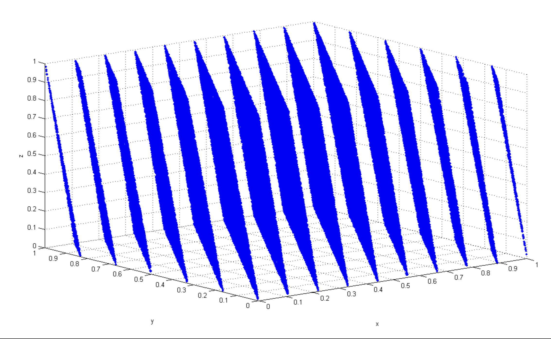
Define the points

$$\pi_1=\left(u_1, \ldots, u_n\right), \pi_2=\left(u_2, \ldots, u_{n+1}\right), \pi_3=\left(u_3, \ldots, u_{n+2}\right), \ldots$$

on a unit -cube formed from successive terms of the sequence of . With such a multiplicative number generator, all -tuples of resulting random numbers lie in at most hyperplanes.

6.1.2 Mersenne Twister

Basic idea:

The generator maintains a state of 624 integers, each 32 bits in size, which is referred to as the state vector. The core idea behind the “twisting” is the application of a transformation function to the state vector.

The state undergoes a series of bitwise operations (such as XOR and shifting) to combine the current state into a new value.

Once the state is initialized, the Mersenne Twister generates pseudorandom numbers by extracting bits from the state vector. These numbers are generated sequentially, and the state vector is updated after each number is produced using the twisting transformation.

$$x_k:=x_{k-(n-m)} \oplus\left(\left(x_{k-n}{ }^u \mid x_{k-(n-1)}{ }^l\right) A\right) \quad k=n, n+1, n+2, \ldots$$ $$\boldsymbol{x} A= \begin{cases}\boldsymbol{x} \gg 1 & x_0=0 \\ (\boldsymbol{x} \gg 1) \oplus \boldsymbol{a} & x_0=1\end{cases}$$ $$\begin{aligned} & y \equiv x \oplus((x \gg u) \& d) \\ & y \equiv y \oplus((y \ll s) \& b) \\ & y \equiv y \oplus((y \ll t) \& c) \\ & z \equiv y \oplus(y \gg l) \end{aligned}$$

6.2 Monte Carlo Method

6.2.1 Direct Sampling

6.2.1.1 Continuous Variable

Basic idea: the random number of the distribution we want is generated by a given function transformation.

$$Q(X)=\int_a^X P(x) d x=\xi$$

If we regard as a random variable, then it satisfies a unitary distriution. Then, we can get the distribution of by calculating

Box-Muller Method:

$$\begin{aligned} & x=\cos \left(2 \pi r_1\right) \times \sqrt{-2 \ln \left(1-r_2\right)} \\ & y=\sin \left(2 \pi r_1\right) \times \sqrt{-2 \ln \left(1-r_2\right)} \end{aligned}$$

6.2.1.2 Discrete Variable

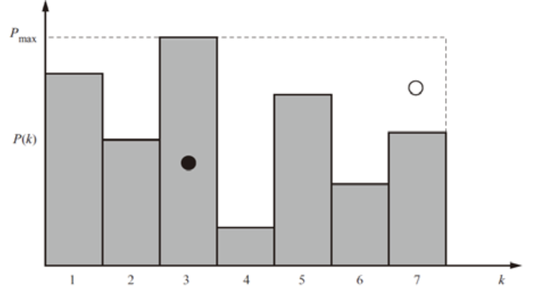
Method 1: use two unitary random variables , the first one determines the position of the point (in which ), and the other determines wether we should accept this point.

Method 2: use only one random variable , and we decide by

$$\sum_{\mathrm{k}=1}^{\mathrm{k}_{\mathrm{r}}-1} P(k) \leq r<\sum_{k=1}^{k_r} P(k)$$

6.2.2 Importance Sampling

Motivation:

We want to use Monte Carlo to compute . There is an event such that is small but is small outside of . When we run the usual Monte Carlo algorithm the vast majority of our samples of will be outside . But outside of is close to zero. Only rarely will we get a sample in where is not small.

Basic idea: Avoid the situation mentioned above by changing the probability distribution of the sample by transforming it. Thus, the variance of statistical results is reduced.

we focus on computing

$$E f(\vec{X})=\int f(\vec{x}) p(\vec{x}) d x$$

The idea of importance sampling is to rewrite the mean as follows. Let be another probability density on such that implies . Then

$$\mu=\int f(x) p(x) d x=\int \frac{f(x) p(x)}{q(x)} q(x) d x$$

We can write the last expression as

$$E_q\left[\frac{f(\vec{X}) p(\vec{X})}{q(\vec{X})}\right]$$

Note that we assumed that whenever .

Advangtage:

Let where is the constant that makes this a probability density. Then for any probability density we have

Since we do not know , we probably do not know either. So the optimal sampling density given in the theorem is not realizable. But again, it gives us a strategy. We want a sampling density which is approximately proportional to .

6.2.3 Reweighting and Correlation Sampling

Basic idea: The idea of reweighting gives rise to the concept of what is called relational sampling, which is calculating the average of two different physical quantities using a set of distributions.

When we sample the distribution and want to calculate the mean value of a function that satisfies the distribution, we can do the following:

$$\langle\langle f(x)\rangle\rangle_Q=\frac{\langle\langle f(x) R(x)\rangle\rangle_P}{\langle\langle R(x)\rangle\rangle_P}$$

where

$$R(x)=W_q(x) / W_p(x)$$

The proof is straightforward:

$$\frac{\int d x f(x) W_q(x)}{\int d x W_q(x)}=\frac{\int d x f(x) R(x) W_p(x)}{\int d x R(x) W_p(x)}$$

Remark:

The requirement of this method is that the weights should be as close as possible, otherwise the convergence of the calculation will become worse; To some extent this is similar to the understanding in importance sampling.

6.3 Markov Chain Monte Carlo Method

Motivation: How to sample a correlated multidimensional distribution?

Basic idea:

A Markov chain is a sequence of random variables where the next state depends only on the current state (not on previous ones). This “memoryless” property is key to MCMC, as it allows us to generate samples step by step based on the current state.

Starting from an initial state, the algorithm generates a sequence of states by applying a transition function that is designed so that, in the long run, the sequence of states will approximate the target distribution.

Key Steps in MCMC:

• Initialization: Start at a random state.
• Sampling: Propose a new state based on the current state.
• Acceptance: Accept the new state with a probability that ensures convergence to the target distribution.
• Repeat: Continue the process for many iterations to generate a sequence of samples.

$$x_{n+1}=F\left(x_n, \xi_n\right)$$

we can get the possibility distribution of

$$\mathrm{P}_{n+1}\left(x^{\prime}\right)=\sum_x P_{j o i n t, n}\left(x^{\prime}, x\right)=\sum_x P\left(x^{\prime} \mid x\right) \mathrm{P}_n(x)$$

6.3.1 Detailed Balance

Motivation: Whether in the evolutionary process can eventually converge to an equilibrium distribution?

When we reach the balance:

$$P_{e q}\left(x^{\prime}\right)=\sum_x P\left(x^{\prime} \mid x\right) P_{e q}(x)$$

If satisfy the following condition:

$$P\left(x^{\prime} \mid x\right) P_{e q}(x)=P\left(x \mid x^{\prime}\right) P_{e q}\left(x^{\prime}\right)$$

which we call it detailed balance condition, can eventually converge to an equilibrium distribution

6.3.2 Convergence to Stationarity

need to be completed

6.3.3 Metropolis-Hastings Algorithm

Basic idea: We decompose conditional probability into two subprocesses ——Test first, then choose whether to accept

$$P\left(x^{\prime} \mid x\right)=T\left(x^{\prime} \mid x\right) A\left(x^{\prime} \mid x\right)$$

In the Metropolis-Hastings algorithm, in fact, the probability of receiving can be expressed as follows

$$A\left(x^{\prime} \mid x\right)=\operatorname{Min}\left\{1, \frac{P\left(x^{\prime}\right) T\left(x \mid x^{\prime}\right)}{P(x) T\left(x^{\prime} \mid x\right)}\right\}$$

This approach can avoid cases where the probability distribution is very steep, and the algorithm will not always reject it, thus increasing the convergence speed.

The Metropolis-Hastings algorithm satisfies the condition of detailed balance.

Convergence to stationarity

$$\lim _{n \rightarrow \infty} \pi_n(x)=P(x)$$

We consider that the contribution of comes from both the accepted events that evolve from to and the rejected events that evolve from to .

$$\pi_{n+1}(x)=\int A\left(x \mid x^{\prime}\right) T\left(x \mid x^{\prime}\right) \pi_n\left(x^{\prime}\right) d x^{\prime}+\pi_n(x) \int\left[1-A\left(x^{\prime} \mid x\right)\right] T\left(x^{\prime} \mid x\right) d x^{\prime}$$

If , then we have

$$\pi_{n+1}(x)=\int A\left(x \mid x^{\prime}\right) T\left(x \mid x^{\prime}\right) P\left(x^{\prime}\right) d x^{\prime}+P(x) \int\left[1-A\left(x^{\prime} \mid x\right)\right] T\left(x^{\prime} \mid x\right) d x^{\prime}$$

use the detailed balance and normalizing condition, we finally get

$$\pi_{n+1}(x)=P(x) \int T\left(x^{\prime} \mid x\right) d x^{\prime}=P(x)$$

Usually we take

$$\mathrm{T}\left(\mathrm{x}^{\prime} \mid \mathrm{x}\right)=\left\{\begin{array}{lr} \frac{1}{\Delta} & \left|x^{\prime}-x\right|<\Delta / 2 \\ 0 & \text { otherwise } \end{array}\right.$$

6.4 Statistical Error Analysis

6.4.1 Average Values and Statistical Errors

$$\sigma_{\mathrm{E}}=\sqrt{\frac{\sum_{i=1}^N\left(E_i-\bar{E}\right)^2}{N(N-1)}}$$

6.4.2 Blocking Analysis

Motivation: In Monte Carlo simulations or other random processes, the sampled data often have a certain degree of autocorrelation, that is, the value of one sample may have some correlation with the value of the previous sample. This affects the estimate of the sample mean and error, as using all the data directly may underestimate the error. Block analysis reduces the effect of autocorrelation by splitting the data into multiple smaller blocks, resulting in more reliable error estimates.

Consider a list of samples, each given the value , and we divide it into segments, each of length .

$$\bar{E}^J=\frac{1}{L} \sum_{i=1}^L E_i$$

then we calculate the average of

$$\bar{E}=\frac{1}{M} \sum_{J=1}^M \bar{E}^J$$

Finally we get the standard deviation

$$\sigma_{\mathrm{E}}=\frac{s_E}{\sqrt{M}}=\sqrt{\frac{\sum_J^B\left(\bar{E}^J-\bar{E}\right)^2}{M(M-1)}}$$

6.4.3 Bootstrap Method

Basic idea: The distribution of sample statistics (such as mean, variance, etc.) is estimated by repeated sampling to derive error estimates and confidence intervals.

Repeat random sampling in the original sample

and then

$$\bar{E}=\frac{1}{M} \sum_{i=1}^M E\left(X_i^B\right)$$

and

$$\sigma_{\mathrm{E}}^B=\sqrt{\frac{\sum_{i=1}^M\left(E\left(X_i^B\right)-\bar{E}\right)^2}{M(M-1)}}$$

6.4.4 Jackknife Method

Basic idea: The core idea of the Jackknife method is to estimate the bias and variance of the statistics by removing one sample point at a time and calculating the statistics based on the remaining samples.

6.5 Monte Carlo Simulation Example

6.5.1 Two-dimension Ising Model

Basic idea: need to be completed

6.5.1.1 General Condition

$$\mathrm{U}=-\sum_{i, j \in \text { neighbors }} J \sigma_i \sigma_j$$

the total acceptance possibility is

$$A\left(\Omega^{\prime} \mid \Omega\right)=\operatorname{Min}\left\{1, e^{-\beta[U(v)-U(\mu)]}\right\}$$

where

$$U(v)-U(\mu)=2 J \sum_{i \in \text { n.n.of } k} \sigma_i^\mu \sigma_{\mathrm{k}}^\mu=2 J \sigma_{\mathrm{k}}^\mu \sum_{i \in \text { n.n.of } k} \sigma_i^\mu$$

With the above Monte Carlo basic operation, we can count the physical quantities we are interested in, such as

$$c=\frac{\beta^2}{L}\left(\left\langle E^2\right\rangle-\langle E\rangle^2\right)$$ $$\chi=\frac{\beta}{\mathrm{L}^2}\left(\left\langle M^2\right\rangle-\langle M\rangle^2\right)=\beta \mathrm{L}\left(\left\langle m^2\right\rangle-\langle m\rangle^2\right)$$

We use the self-correlation function to see how much length we need to take to do the Monte Carlo simulation is appropriate

$$\chi(t)=\int d t^{\prime}\left[m\left(t^{\prime}\right)-\langle m\rangle\right]\left[m\left(t^{\prime}+t\right)-\langle m\rangle\right]=\int d t^{\prime}\left[m\left(t^{\prime}\right) m\left(t^{\prime}+t\right)-\langle m\rangle^2\right]$$

usually we assume that the self-correlation function has an exponential decay from

$$\chi(t)=\mathrm{e}^{-t/\tau}$$

the fitting parameter is known as correlation time. If we want to get two samples without correlations, then we should choose two points in time with an interval greater than .

In addition to fitting the exponential function, it is actually possible to integrate the correlation function whose integral also converges to the correlation time .

$$\int_0^{+\infty} \frac{\chi(t)}{\chi(0)} d t=\int_0^{+\infty} e^{-t / \tau} d t=\tau$$

In practice, we usually calculate

$$\tau\left(t^{\prime}\right)=\int_0^{t^{\prime}} e^{-t / \tau} d t$$

and it’s discrete form is

$$\begin{aligned} \chi(t)= & \frac{1}{t_{\max }-t+1} \sum_{t^{\prime}=0}^{t_{\max }-t} m\left(t^{\prime}\right) m\left(t^{\prime}+t\right) \\ & \quad-\frac{1}{t_{\max }-t+1} \sum_{t^{\prime}=0}^{t_{\max }-t} m\left(t^{\prime}\right) \times \frac{1}{t_{\max }-t} \sum_{t^{\prime}=0}^{t_{\max }-t} m\left(t^{\prime}+t\right) \end{aligned}$$

or we can calculate with the help of Fourier transformation

$$\begin{aligned} \tilde{\chi}(\omega)=\int d t & e^{i \omega t} \int d^{t^{\prime}}\left[m\left(t^{\prime}\right)-\langle m\rangle\right]\left[m\left(t^{\prime}+t\right)-\langle m\rangle\right] \\ & =\int d t \int d t^{\prime} e^{-i \omega t}\left[m\left(t^{\prime}\right)-\langle m\rangle\right] e^{i \omega\left(t^{\prime}+t\right)}\left[m\left(t^{\prime}+t\right)-\langle m\rangle\right]=\widetilde{m}^{\prime}(\omega) \widetilde{m}^{\prime}(-\omega) \\ & =\left|\widetilde{m}^{\prime}(\omega)\right|^2 \end{aligned}$$

Additionally, we can easily show that the correlation time corresponds to the eigenvalue of the Markov matrix

$$\tau_i=-\frac{1}{\log \lambda_i}, \quad i \neq 0$$

Except the self-correlation function, we can also define so-called two-body correlation function

$$G_c^{(2)}(i, j)=\left\langle\sigma_i \sigma_j\right\rangle-\left\langle\sigma_i\right\rangle\left\langle\sigma_j\right\rangle=\left\langle\sigma_i \sigma_j\right\rangle-m^2$$

which we can calculate by the following form

$$G_c^{(2)}(r)=\frac{1}{N} \sum_{r_j-r_i=r}\left[\left\langle\sigma_i \sigma_j\right\rangle-m^2\right]$$

or the Fourier transformation method

$$\begin{aligned} \tilde{G}_c^{(2)}(k)=\sum_r & e^{i k \cdot r} G_c^{(2)}(r)=\frac{1}{N} \sum_r \sum_{r_j-r_i=r} e^{i k \cdot\left(r_j-r_i\right)}\left[\left\langle\sigma_i \sigma_j\right\rangle-m^2\right] \\ = & \frac{1}{\mathrm{~N}}\left\langle\sum_{r_i} e^{-i k \cdot r_i}\left(\sigma_i-m\right) \sum_{r_j} e^{i k \cdot r_j}\left(\sigma_i-m\right)\right\rangle=\frac{1}{N}\langle | \tilde{\sigma}^{\prime}(k) |^2 \rangle \end{aligned}$$

6.5.1.2 Monte Carlo Simulation Near Critical Temperature

Basic idea: Clustering flipping algorithm, Flipping too slowly one by one, flipping a large number of related grid points at a time, is called a cluster

How to define a cluster?

Key point: First randomly select a point, and then extend the connection outward, the connection probability satisfies

$$P_{i j}=1-\mathrm{e}^{-2 \beta J}$$

The reason why we take in this form is that we can easily show the following relation

$$\frac{A\left(x^{\prime} \mid x\right)}{A\left(x \mid x^{\prime}\right)}=\left[e^{2 \beta J}\left(1-P_{\text {bond }}\right)\right]^{n-m}$$

where the process from breaks keys and the process from breaks keys. Then

$$\frac{A\left(x^{\prime} \mid x\right)}{A\left(x \mid x^{\prime}\right)}=1$$

Therefore, we can take

$$A(x'|x)=A(x|x')=1$$

We can avoid talking about the acceptance probability.

• Swendsen-Wang Algorithm

​ All clusters flip simultaneously with a probability of 1/2

• Wolff Algorithm

​ Only one cluster is found at a time, and this cluster must be flipped

6.5.2 Spatial Distribution of Particles

Basic idea: the final equvilibrium distribution is given by the partition function, and the use the Metropolis method

6.5.2.1 Canonical Ensemble

If we want to know the statistic properties of a group of particles , first we should write down the partition function of this system (if the temperature is fixed)

$$Q(N, V, T)=\frac{1}{N!\lambda^{3 N}} \int d \vec{r} e^{-\beta U(\vec{r})}$$

and

$$\mathrm{P}(\vec{r}) \propto e^{-\beta U(\vec{r})}$$

using the Metropolis method to sampling, we can define the acception possibility

$$\mathrm{A}\left(\overrightarrow{\mathrm{r}}^{\prime} \mid \vec{r}\right)=\operatorname{Min}\left\{1, e^{-\beta\left[U\left(\vec{r}^{\prime}\right)-U(\vec{r})\right]}\right\}$$

which means when the total potential decreases, we must accept this transition.

In each step, we just move one particle with an appropriate step length which leads to about 50% accept possibility (since we move all particles will induce a vary large change of potential, leading to a vary low accept possibility)

$$\vec{r}_i^{\prime}-\vec{r}_i=\delta \vec{e}_i$$

6.5.2.2 Volume is Not Fixed

If the volume is not fixed, we can rewrite the partition function

$$\Delta(\mathrm{N}, \mathrm{P}, \mathrm{~T})=\frac{1}{\mathrm{~V}_0 N!\lambda^{3 N}} \int_0^{\infty} d V e^{-\beta P V} V^N \int d \vec{s}_1 \ldots d \vec{s}_N e^{-\beta U\left(V^{\frac{1}{3}} \vec{s}_1, \ldots, V^{\frac{1}{3}} \vec{s}_N\right)}$$

then

$$\mathrm{P}(s) \propto \mathrm{e}^{-\beta P V} e^{-\beta U} e^{N \ln V}$$

acceptance possibility

$$\mathrm{A}\left(V^{\prime} | V\right)=\min \left[1, \mathrm{e}^{-\beta \mathrm{P}\left(\mathrm{~V}^{\prime}-V\right)} e^{-\beta\left(U^{\prime}-U\right)} e^{N \ln \left(V^{\prime} / V\right)}\right]$$

6.5.2.3 Grand Canonical Ensemble

$$\mathrm{Z}(\mu, \mathrm{~V}, \mathrm{~T})=\sum_{\mathrm{N}=0}^{\infty} e^{\beta \mu N} \frac{1}{N!\lambda^{3 N}} \int d \vec{r}_1 \ldots d \vec{r}_N e^{-\beta U(\vec{r})}$$

Then we have

$$\mathrm{A}(\mathrm{~N}+1 \mid \mathrm{N})=\min \left[1, \frac{\mathrm{~V}}{\lambda^3(N+1)} \mathrm{e}^{\beta \mu} \mathrm{e}^{-\beta\left(\mathrm{U}^{\prime}-U\right)}\right]$$ $$\mathrm{A}(\mathrm{~N}-1 \mid \mathrm{N})=\min \left[1, \frac{\lambda^3 N}{V} \mathrm{e}^{-\beta \mu} \mathrm{e}^{-\beta\left(\mathrm{U}^{\prime}-U\right)}\right]$$

6.5.3 Solve Differential Equation by Monte Carlo Method

Basic idea: need to be completed

Advantage: The statistical error decreases with the increase of the number of Monte Carlo samples and does not depend on the dimension of the space.

6.5.3.1 Walk on Spheres Method

Basic idea: the solution inside the region relates to that on boundary.

Consider an arbitary dimension Laplace’s equation

$$\begin{array}{lc} \Delta u(x)=0 & x \in \Omega \\ u(x)=f(x) & x \in \Gamma \end{array}$$

An important relation is

$$u(x)=E_x\left[f\left(x_{\Gamma}\right)\right]$$

(the institutive interpretation of this relation is the balance of a diffusion process)

The symbol represents the evolution from to on the boundary through a random process.

What about a random process —— Walk on Spheres

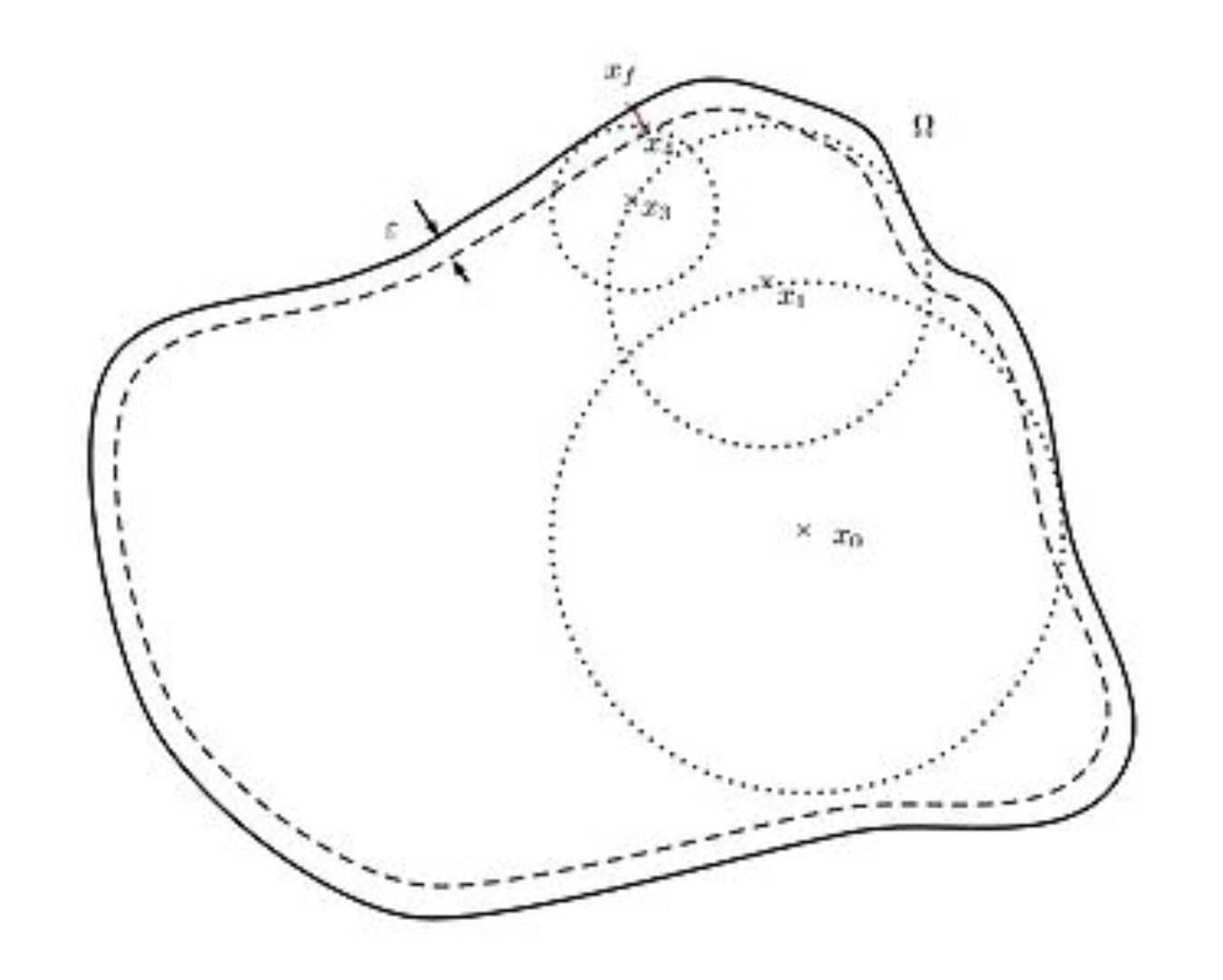
the dash line in the picture denotes the cut-off region.

6.5.3.2 Green’s Function Method

Basic idea: treat all 𝑓 as a set of many point sources whose potential field 𝑢 is the integral of its product with its Green’s function. The specific operation is modeled after the previous discussion, that is, a random point source is generated according to the distribution of point source, and the potential field generated at is calculated.

Another method to cut-off ——Green’s function first passage

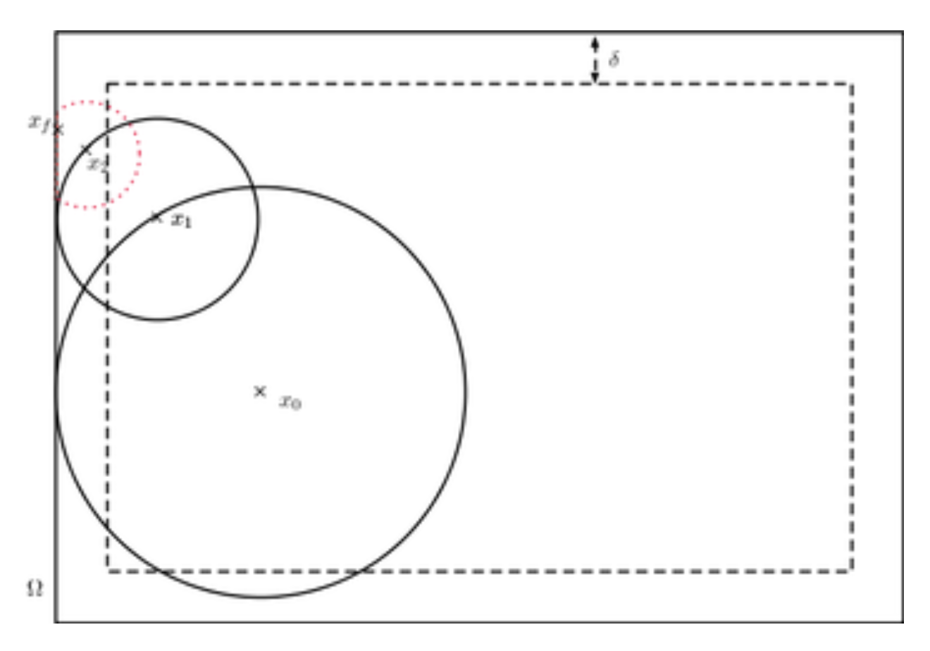
the radius of the red sphere is .

Now let’s consider a general differential equation

$$\hat{L}(x) u(x)=f(x)$$

the Green’s function satisfies

$$\widehat{L}(x) G\left(x, x^{\prime}\right)=\delta\left(x-x^{\prime}\right)$$

and the solution is

$$u(x)=\int G\left(x, x^{\prime}\right) f\left(x^{\prime}\right) d x^{\prime}$$

Considering the first coundary condition, the solution can be wriiten as

$$u(x)=\int G\left(x, x^{\prime}\right) f\left(x^{\prime}\right) d x^{\prime}-\int \phi \frac{\partial G}{\partial \vec{n}} d S$$

The so-called Green function first channel method is actually a process that requires a special Green function under given boundary conditions and then uses it to sample.

6.5.3.3 Initial-value Problem

$$\frac{\partial \rho(x, t)}{\partial t}=D \nabla^2 \rho(x, t)$$

the Green’s function is given by

$$G\left(x, x^{\prime} ; t, t^{\prime}\right)=\frac{1}{\sqrt{4 \pi D\left(\mathrm{t}-\mathrm{t}^{\prime}\right)}} \exp \left[-\frac{\left(x-x^{\prime}\right)^2}{4 \mathrm{D}\left(\mathrm{t}-\mathrm{t}^{\prime}\right)}\right]$$

the solution is

$$\rho(x, t)=\int \rho\left(x^{\prime}, t^{\prime}\right) G\left(x, x^{\prime} ; t, t^{\prime}\right) d x^{\prime}$$

We can regard this relation as an implicit recursion

$$\rho(x, t+\Delta t)=\int \rho(x', t) G\left(x^{\prime} \rightarrow x ; \Delta t\right) d x^{\prime}$$

We can define walker and it’s a classic random walk with the distribution of .

6.5.4 Quantum Mento Carlo

Basic idea: Shrodinger equation is also a differential equation

$$\mathrm{E}=\int \Psi^*(x) \widehat{H} \Psi(x) d R$$

Naturally, we can choose sampling distribution

$$\mathrm{P}(x)=|\Psi(x)|^2$$

then

$$\mathrm{E}=\int P(x) E_{l o c}(x) d x$$

where

$$E_{l o c}(x)=\Psi^{-1}(x) \widehat{H} \Psi(x)$$

the integral can be discrete

$$\mathrm{E}=\lim _{M \rightarrow \infty} \frac{1}{M} \sum_i^M E_{l o c}\left(x_i\right)$$

Then, how do we optimize the wave function. Note that in the variation principle, we have

$$\mathrm{E}_{\mathrm{T}}=\int \Psi_{\mathrm{T}}^*(x) \widehat{H} \Psi_{\mathrm{T}}(x) d x \geq \mathrm{E}_0=\int \Psi_0^*(x) \widehat{H} \Psi_0(x) d x$$

Suppose the wave function can be described by a parameter

$$\Psi_{\mathrm{T}}(x ; \theta)$$

Our goal is to find a appropriate leading the lowest total energy.

But how to ansatz the form of ? ——approximation only (key issue).

6.5.4.2 Virtual Time Evolution Method

Basic idea:

let , then the solution of Shrodinger equation can be written as

$$\Psi(x, \tau)=e^{-\tau \hat{H}} \Psi(x, 0)$$

Denote

$$\widehat{\mathrm{P}}=\exp (-\tau \widehat{H})$$

We can get an iteration relation

$$\left|\Psi^{k+1}\right\rangle=\widehat{P}\left|\Psi^k\right\rangle$$

use a set of complementary basis to express the state and the operator

$$|\Psi\rangle=\sum_i\left|\Phi_i\right\rangle\left\langle\Phi_i \mid \Psi\right\rangle$$ $$\exp (-\tau \widehat{H})=\sum_i\left|\Phi_i\right\rangle \exp \left(-\tau E_i\right)\left\langle\Phi_i\right|$$

then

$$\begin{aligned} & \lim _{\tau \rightarrow \infty} \exp [-\tau(\widehat{H})]\left|\Psi_{\text {init }}\right\rangle=\lim _{\tau \rightarrow \infty} \sum_i\left|\Phi_i\right\rangle \exp \left[-\tau\left(\mathrm{E}_{\mathrm{i}}\right)\right]\left\langle\Phi_i \mid \Psi_{\text {init }}\right\rangle \\ &=\lim _{\tau \rightarrow \infty}\left|\Phi_0\right\rangle \exp \left[-\tau\left(\mathrm{E}_0\right)\right]\left\langle\Phi_0 \mid \Psi_{\text {init }}\right\rangle+\lim _{\tau \rightarrow \infty}\left|\Phi_1\right\rangle \exp \left[-\tau\left(\mathrm{E}_1\right)\right]\left\langle\Phi_1 \mid \Psi_{i n i t}\right\rangle \\ &+\cdots \approx \lim _{\tau \rightarrow \infty}\left|\Phi_0\right\rangle \exp \left[-\tau\left(\mathrm{E}_0\right)\right]\left\langle\Phi_0 \mid \Psi_{\text {init }}\right\rangle \end{aligned}$$

Which is known as projection algorithm.

We can also use the Green’s function method

$$\mathrm{G}\left(\mathrm{x} \leftarrow \mathrm{x}^{\prime}, \tau\right)=(2 \pi \tau)^{-\frac{3 N}{2}} \exp \left[-\frac{\left(x-x^{\prime}\right)^2}{2 \tau}\right] \times \exp \left[-\frac{\tau\left[U(x)+U\left(x^{\prime}\right)-2 E_T\right]}{2}\right]$$

where the third term means that the number of propagators in the propagation process needs to be “renormalized” in a certain way, which can be realized by the process of extinction/replication of propagators in the specific algorithm implementation.

6.6 Stochastic Differential Equation

The most common form of SDEs in the literature is an ordinary differential equation with the right hand side perturbed by a term dependent on a white noise variable.

For example:

• Lorenz-Haken equations
• Langevin equation
• Karkar-porisi-Zhang
• Black-Scholos

6.6.1 Langevin Equation

$$dx=\mu(x,t)dt+\sigma(x,t)dB_t$$ $$B_t=\int_0^t \xi(t')dt'$$

we have

$$\mathbb{E}[B_t]=0;\quad \mathbb{E}[B_t^2]=t$$ $$\mathbb{E}[B_tB_s]=\text{min}(t,s)$$ $$\mathbb{E}[(B_t-B_s)^2]=|t-s|$$ $$B_t \sim N(0,t)$$ $$B_t^2\sim \chi(t,2t^2)$$

Ito Lemma:

$$X\rightarrow Y(X,t)$$

Then

$$dY=\frac{\partial Y}{\partial t}dt+\frac{\partial Y}{\partial x}dx+\frac{1}{2}\frac{\partial^2 Y}{\partial x^2}(dx)^2$$

There’s an extra second-order term here.

$$(dx)^2=\mu^2dt^2+2\mu\sigma dtdB_t+\sigma^2(dB_t)^2$$

where

$$dB_t\sim N(0,dt)$$ $$(dB_t)^2\sim \chi(t,3dt^2)\approx dt$$

then

$$dY=\frac{\partial Y}{\partial t}dt+\frac{\partial Y}{\partial x}(\mu dt+\sigma dB_t)+\frac{\sigma^2}{2}\frac{\partial^2 Y}{\partial x^2}dt$$

For example:

$$Y=x^2\quad dY=(2x\mu+\sigma^2)dt+2\sigma xdB_t$$ $$x=B_t\quad dY=(2B_t\mu+\sigma^2)dt+2\sigma B_t dB_t$$

then

$$I_t=2\sigma \int_0^t B_t dB_t$$ $$\mathbb{E}[B_tdB_t]=0$$

From

$$\mathbb{E}[(B_{t+dt}-B_t)^2]=dt$$

we can derive

$$\mathbb{E}[B_{t+dt}B_t]=t$$

similarly

$$\mathbb{E}[B_{t}B_{t-dt}]=t-dt$$

If we choose the forward differential, then we have

$$\mathbb{E}[B_tdB_t]=0$$

But if we choose the backward differential and central differential, Then respectively give

$$\mathbb{E}[B_tdB_t]_{\text{back}}=dt$$ $$\mathbb{E}[B_tdB_t]_{\text{central}}=dt/2$$

We can find that it’s asymmetrical! It illustrates the importance of Ito Lemma.

6.6.2 Euler-Maruyuma Method