Computational Physics (Part1)

[TOC]

1. Interpolation

1.1 Polynomial Interpolation

1.1.1 Lagrange Polynomials

basic ideal: each term

$L_i(x_k)=\delta_{i,k}$

The final formula is:

$p(x)=\sum_{i=0}^{n}f_i\prod_{k=0,k\neq i}^{n}\frac{x-x_k}{x_i-x_k}$

1.1.2 Barycentric Lagrange Interpolation

motivation: Essentially the same as Lagrange interpolation, but the time complexity is reduced from to .

define two quantities:

$\omega(x)=\prod_{i=0}^{n}(x-x_i)$

and

$u_i=\frac{1}{\prod_{k=0,k\neq i}^{n}(x_i-x_k)}$

The final formula is:

$p(x)=\omega(x)\sum_{i=0}^n f_i\frac{u_i}{x-x_i}$

Since we only need to compute once, and each computation only needs to compute the terms in and summation, the time complexity is only .

1.1.3 Newton’s Divided Difference

Basic idea: Starting from a sample point, the number of sample points is gradually increased and the interpolation is completed by adding higher order terms without changing the original difference polynomial. At this time, the new coefficient and the original old coefficient satisfy a specific recurrence relationship

Define a function:

$f[x_1x_2\cdots x_r]=\sum_{k=1}^r \frac{f(x_k)}{\prod_{i\neq k}(x_k-x_i)}$

It can also be defined recursively by

$f[x_1x_2\cdots x_{r-1}x_r]=\frac{f[x_1x_2\cdots x_{r-1}]-f[x_2\cdots x_r]}{x_1-x_k}$

The final formula is:

$p(x)=f(x_0)+f[x_1x_0](x-x_0)+f[x_2x_1x_0](x-x_0)(x-x_1)+\cdots+f[x_nx_{n-1}\cdots x_0](x-x_0)\cdots (x-x_n)$

Recurrence diagram

$\begin{array}{ccccc} f_0 & & \\ f_1 & f\left[x_0 x_1\right] & \\ \vdots & \vdots & \ddots & \\ f_{n-1} & f\left[x_{n-2} x_{n-1}\right] & f\left[x_{n-3} x_{n-2} x_{n-1}\right] \cdots & f\left[x_0 \cdots x_{n-1}\right] \\ f_n & f\left[x_{n-1} x_n\right] & f\left[x_{n-2} x_{n-1} x_n\right] & \cdots & f\left[x_1 \cdots x_n\right] \quad f\left[x_0 \cdots x_n\right] \end{array}$

1.1.4 Neville Method

Basic idea: It’s also recursion, but in a different way (interpolating recursion from both ends).

The final formula:

$P_{0,1\ldots k}(x)=\frac{(x-x_0)P_{1\ldots k}(x)-(x-x_k)P_{0\ldots k-1}(x)}{x_k-x_0}$

1.2 Spline Interpolation

Motivation: Polynomials are not well suited for interpolation over a large range

Basic idea: Often spline functions are superior which are piecewise defined polynomials. After we have chosen the degree of the polynomial, all we need to do is determine the continuity condition.

1.2.1 Cubic Spline

We use third-order polynomials for interpolation

$p_i(x)=\alpha_i+\beta_i(x-x_i)+\gamma_i(x-x_i)^2+\delta_i(x-x_i)^3$

Boundary Conditions:

$i=0\cdots n-1\\ p_i(x_{i+1})=p_{x+1}(x_{i+1})\\ p_i'(x_{i+1})=p_{x+1}'(x_{i+1})\\ p_i''(x_{i+1})=p_{x+1}''(x_{i+1})\\$

For and , the most common choice are natural boundary conditions:

$s''(x_0)=s''(x_n)=0$

Define

$M_i=s''(x_i)\\ h_{i+1}=x_{i+1}-x_i$

So we can write

$p_i''(x)=M_{i+1}\frac{(x-x_i)}{h_{i+1}}+M_i\frac{(x_{i+1}-x)}{h_{i+1}}$

And then we can go through the integration, and then we can determine the coefficients based on the boundary conditions.

The final formula:

$\alpha_i=y_i\\ \beta_i=\frac{y_{i+1}-y_i}{h_{i+1}}-h_{i+1}\frac{M_{i+1}+2M_i}{6}\\ \gamma_i = \frac{M_i}{2}\\ \delta_i = \frac{M_{i+1}-M_i}{6h_{i+1}}$

can be solved by a system of linear equations:

$\left[\begin{array}{cccccc} 2 & \lambda_1 & & & & \mu_1 \\ \mu_2 & 2 & \lambda_2 & & & \\ & \mu_3 & 2 & \lambda_3 & & \\ & & \ddots & \ddots & \ddots & \\ & & & \mu_{n-1} & 2 & \lambda_{n-1} \\ \lambda_n & & & & \mu_n & 2 \end{array}\right]\left[\begin{array}{c} M_1 \\ M_2 \\ M_3 \\ \vdots \\ M_{n-1} \\ M_n \end{array}\right]=\left[\begin{array}{c} d_1 \\ d_2 \\ d_3 \\ \vdots \\ d_{n-1} \\ d_n \end{array}\right]$

1.4 Rational Interpolation

1.4.1 Pade Approximant

Basic idea: Using rational function to fit McLaurin series

$R_{M/N}=\frac{P_M(x)}{Q_N(x)}$

Which reproduces the McLaurin series of

$f(x)=a_0+a_1x+a_2x^2+\cdots$

up to order M+N, i.e.

$\begin{aligned} &\begin{aligned} & p_0=q_0 a_0 \\ & p_1=q_0 a_1+q_1 a_0 \\ & p_2=q_0 a_2+a_1 q_1+a_0 q_2\\ .\\ .\\ . \end{aligned}\\ &\begin{aligned} & p_M=q_0 a_M+a_{M-1} q_1+\cdots+a_0 q_M \\ & 0=q_0 a_{M+1}+q_1 a_M+\cdots+q_N a_{M-N+1}\\ .\\ .\\ . \end{aligned}\\ &0=q_0 a_{M+N}+q_1 a_{M+N-1}+\cdots+q_N a_M \end{aligned}$

1.4.2 Barycentric Rational Interpolation

Remark:

$R(x)=\frac{\sum_{i=0}^n f_i\frac{u_i}{x-x_i}}{\sum_{i=0}^n \frac{u_i}{x-x_i}}$

it becomes a rational function if we take as general parameters (obviously can not be zero)

and

$\lim_{x\rightarrow x_i}R(x)=f_i$

We can obtain two polynomials

$P(x)=\sum_{i=0}^n u_i f_i \prod_{j=0 ; j \neq i}^n\left(x-x_j\right)=\sum_{i=0}^n u_i f_i \frac{\omega(x)}{x-x_i}$ $Q(x)=\sum_{i=0}^n u_i \prod_{j=0 ; j \neq i}^n\left(x-x_j\right)=\sum_{i=0}^n u_i \frac{\omega(x)}{x-x_i}$

a rational interpolating function is given by

$R(x)=\frac{P(x)}{Q(x)}$

1.5 Multivariate Interpolation

1.5.1 Bilinear Interpolation

It can be written as a two dimensional polynomial

$p\left(x_i+h_x, y_i+h_y\right)=a_{00}+a_{10} h_x+a_{01} h_y+a_{11} h_x h_y$

with

$\begin{aligned} a_{00} & =f\left(x_i, y_i\right) \\ a_{10} & =\frac{f\left(x_{i+1}, y_i\right)-f\left(x_i, y_i\right)}{x_{i+1}-x_i} \\ a_{01} & =\frac{f\left(x_i, y_{i+1}\right)-f\left(x_i, y_i\right)}{y_{i+1}-y_i} \\ a_{11} & =\frac{f\left(x_{i+1}, y_{i+1}\right)-f\left(x_i, y_{i+1}\right)-f\left(x_{i+1}, y_i\right)+f\left(x_i, y_i\right)}{\left(x_{i+1}-x_i\right)\left(y_{i+1}-y_i\right)} \end{aligned}$

1.5.2 Two-Dimensional Spline Interpolation

Basic idea:

$f_{i,j}=f(ih_x,jh_y)$

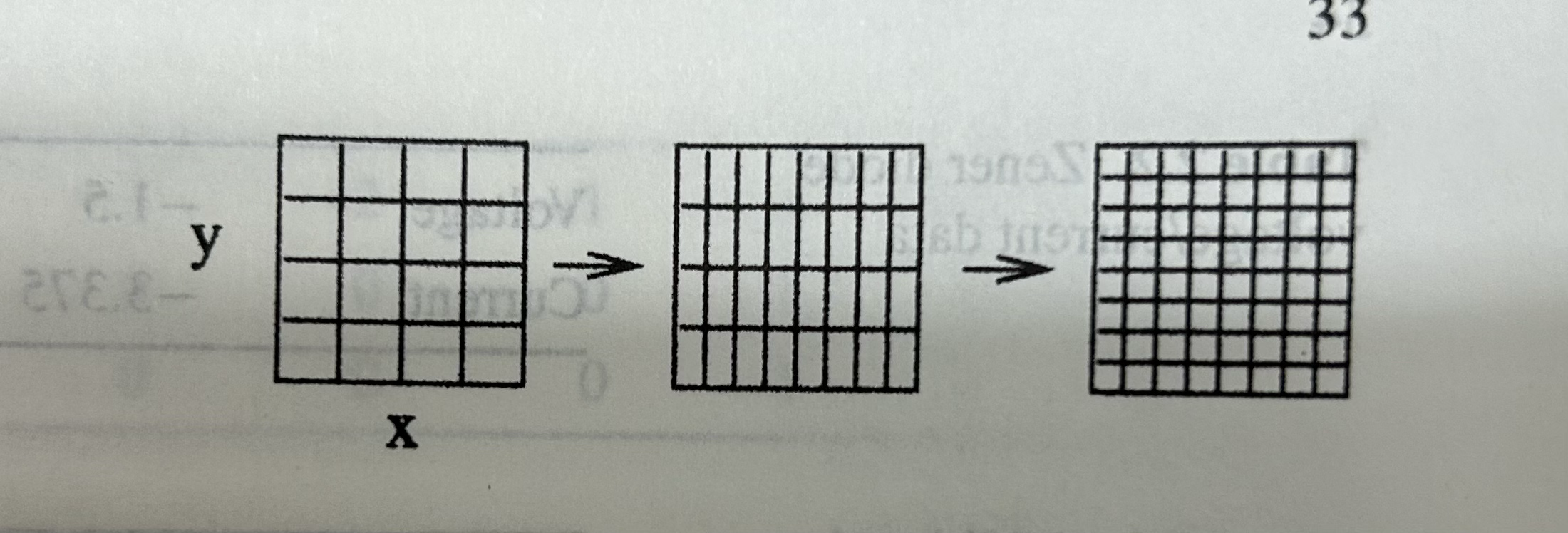
First, for each , we calculate new data sets of

$f_{i',j}=s(x_{i'},f_{ij},i\leq i<N_x)$

Then, for each $i’$, we calculate new data sets of y

$f_{i',j'}=s(y_{j'},f_{i'j},0\leq j<N_y)$

1.6 Chebyshev polynomial

the function can be approximated by the trigonometry polynomial with $N=2M,T=2\pi$

$f(\cos t)=\frac{1}{2 M} c_0+\frac{1}{M} \sum_{j=1}^{M-1} c_j \cos (j t)+\frac{1}{2 M} c_M \cos (M t)$

Which interpolates at the sample points

$\begin{aligned} t_n=n \Delta t & =n \frac{\pi}{M} \quad \text { with } n=0,1 \cdots M \\ x_n & =\cos t_n=\cos \left(n \frac{\pi}{M}\right) \end{aligned}$

the Fourier coefficient are given by

$c_j=f_0+2 \sum_{n=1}^{M-1} f\left(\cos \left(t_n\right)\right) \cos \left(\frac{\pi}{M} j n\right)+f_M \cos (j \pi)$

define

$T_j(x)=\cos (j \arccos (x))$

And can be calculated recursively

$\begin{aligned} & T_0(x)=1 \\ & T_1(x)=x \\ T_{j+1}(x)= & 2 x T_j(x)-T_{j-1}(x) \end{aligned}$

Hence the Fourier series corresponding to a Chebyshev approximation

$f(x)=\sum_{j=0}^M a_j T_j(x)=\frac{c_0}{2 M} T_0(x)+\sum_{j=1}^{M-1} \frac{c_j}{M} T_j(x)+\frac{c_M}{2 M} T_M(x)$

2. Numerical Differentiation

2.1 One-Sided Difference Quotient

Forward:

$\frac{\Delta f}{\Delta x}=\frac{f(x+h)-f(x)}{h}$

Backward:

$\frac{\Delta f}{\Delta x}=\frac{f(x)-f(x-h)}{h}$

truncation error:

$\frac{f(x+h)-f(x)}{h}=f'(x)+\frac{h}{2}f''(x)+\cdots$

2.2 Central Difference Quotient

$\frac{\Delta f}{\Delta x}=\frac{f(x+h/2)-f(x-h/2)}{h}=f'(x)+\frac{h^2}{24}f'''(x)$

2.3 Extrapolation Methods

Basic idea: Higher order errors are eliminated by using the low order derivative approximation of asynchronously long lengths, thus achieving higher accuracy (use the method of interpolation)

define:

$D(x)=\frac{f(x+h)-f(x-h)}{2h}=f'(x)+\frac{h^2}{3!}f'''(x)+\frac{h^4}{5!}f^{(5)}(x)+\cdots$

we choose:

$h_{i+1}=\frac{h_i}{2}$

If we want to eliminate the term, we can use the polynomial of degree 1 (with respect to )

$p(h)=a+b(h^2)$

Using the Lagrange method

$p(h)=D_0 \frac{h^2-\frac{h_0^2}{4}}{h_0^2-\frac{h_0^2}{4}}+D_1 \frac{h^2-h_0^2}{\frac{h_0^2}{4}-h_0^2} .$

Extrapolation for gives

$p(0)=-\frac{1}{3}D_0+\frac{4}{3}D_1=f'(x)-\frac{1}{4}\frac{h_0^4}{5!}f^{(5)}(x)+\cdots$

Neville method

Based on the above interpolation ideas, we can introduce the Neville method,

$P_{i \cdots k}\left(h^2\right)=\frac{\left(h^2-\frac{h_0^2}{2}\right) P_{i+1 \cdots k}\left(h^2\right)-\left(h^2-\frac{h_0^2}{2^2}\right) P_{i \cdots k-1}\left(h^2\right)}{\frac{h_0^2}{2^k}-\frac{h_0^2}{2}}$

gives for

$P_{i \cdots k}=\frac{P_{i \cdots k-1}-2^{k-i} P_{i+1 \cdots k}}{1-2^{k-i}}$

2.4 Higher Derivatives

Basic idea: Difference quotients for higher derivatives can be obtained systematically using polynomial interpolation.

Process:

choose , such as
$x_0-2h,x_0-h,x_0,x_0+h,x_0+2h$
calculate the polynomial using the method of interpolation;
calculate the derivative of the polynomial to obtain the difference quotient we need.

2.5 Partial Derivatives of Multivariate Function

Basic idea: the same as higher derivatives, we can use the polynomial approximation

two-dimension Lagrange interpolation

$L_{i, j}(x, y)=\prod_{k \neq i} \frac{\left(x-x_k\right)}{\left(x_i-x_k\right)} \prod_{j \neq l} \frac{\left(y-y_l\right)}{\left(y_j-y_l\right)}$

The interpolating polynomial is

$p(x, y)=\sum_{i, j} f_{i, j} L_{i, j}(x, y) .$

After we obtain the polynomial, we can calculate the partial derivatives of such as,

$\text{grad}f(x_0,y_0)\approx \text{grad} p(x_0,y_0)$

3. Numerical Integration

In generaal a definite integral can be approximated numerically as the weighted average over a finite number of function values

$\int_{a}^{b}f(x)dx\approx \sum_{x_i}w_i f(x_i)$

3.1 Equidistant Sample Points

Basic idea: Equidistant Sample points, just like it’s name said, and plus the interpolation polynomial approximation

$x_i=a+i h \quad i=0 \cdots N \quad h=\frac{b-a}{N}$

Lagrange method

$p(x)=\sum_{i=0}^N f_i \prod_{k=0, k \neq i}^N \frac{x-x_k}{x_i-x_k}$

Integration of the polynomial gives

$\int_a^b p(x) d x=\sum_{i=0}^N f_i \int_a^b \prod_{k=0, k \neq i}^N \frac{x-x_k}{x_i-x_k} d x$ $\int_a^b \prod_{k=0, k \neq i}^N \frac{x-x_k}{x_i-x_k} d x=\int_0^N \prod_{k=0, k \neq i}^N \frac{s-k}{i-k} h d s=h \alpha_i$

and hence

$\int_a^b p(x) d x=(b-a) \sum_{i=0}^N f_i \alpha_i .$

Using the same method, we can obtain more accurate approximation formula

3.1.1 Closed Newton-Cotes Formula

gives the trapezoidal rule

$h\frac{f_0+f_1}{2}$

gives Simpson’s rule

$2 h \frac{f_0+4 f_1+f_2}{6}$

Larger give further integration rules

$\begin{gathered} 3 h \frac{f_0+3 f_1+3 f_2+f_3}{8} \\ 4 h \frac{7 f_0+32 f_1+12 f_2+32 f_3+7 f_4}{90} \\ 5 h \frac{19 f_0+75 f_1+50 f_2+50 f_3+75 f_4+19 f_5}{288} \end{gathered}$

Milne-rule

$6 h \frac{41 f_0+216 f_1+27 f_2+272 f_3+27 f_4+216 f_5+41 f_6}{840}$

Weddle-rule.

3.1.2 Open Newton-Cotes Formula

Alternatively, the integral can be computed form only interior points

$x_i=a+ih\quad i=1,2\cdots N\quad h=\frac{b-a}{N+1}$

3.1.3 Composite NewTon-Cotes Rules

Basic idea: divided the integration range into small sub-intervals

$\left[x_i, x_{i+1}\right] \quad x_i=a+i h \quad i=0 \cdots N$

trapezoidal rule ()

$T=h\left(\frac{f(a)}{2}+f(a+h)+\cdots+f(b-h)+\frac{f(b)}{2}\right)$

Simpson’s rule ()

$\begin{aligned} S= & \frac{h}{3}(f(a)+4 f(a+h)+2 f(a+2 h)+4 f(a+3 h)+\cdots \\ & +2 f(b-2 h)+4 f(b-h)+f(b)) \end{aligned}$

Midpoint rule ()

$M=2 h(f(a+h)+f(a+3 h)+\cdots+f(b-h))$

3.1.4 Extrapolation Method (Romberg Integration)

Basic idea: for the trapezoidal rule, we have

$\int_{x_0}^{x_N} f(x) d x-T=\alpha_2 h^2+\alpha_4 h^4+\cdots+\alpha_{2 m-2} h^{2 m-2}+O\left(h^{2 m}\right) .$

we can use points to interpolate. And also we have the Neville method

$P_{i \cdots k}\left(h^2\right)=\frac{\left(h^2-\frac{h_0^2}{2^{2 i}}\right) P_{i+1 \cdots k}\left(h^2\right)-\left(h^2-\frac{h_0^2}{2^{2 k}}\right) P_{i \cdots k-1}\left(h^2\right)}{\frac{h_0^2}{2^{2 k}}-\frac{h_0^2}{2^{2 k}}}$

3.2 Optimized Sample Points

Motivation: the polynomial approximation converges slowly, so we should optimize the sample point positions.

Solution: Using orthogonal complete eigenvector expansion to do approximation, improve the convergence speed, and then improve the accuracy of numerical integration

3.2.1 Clenshaw-Curtis Expressions

Basic idea: use the trigonometric polynomial to approximate

$f(\cos t)=\frac{1}{2 M} c_0+\frac{1}{M} \sum_{j=1}^{M-1} c_j \cos (j t)+\frac{1}{2 M} c_M \cos (M t)$

Which interpolates at the sample points

$\begin{aligned} t_n=n \Delta t & =n \frac{\pi}{M} \quad \text { with } n=0,1 \cdots M \\ x_n & =\cos t_n=\cos \left(n \frac{\pi}{M}\right) \end{aligned}$

the Fourier coefficient are given by

$c_j=f_0+2 \sum_{n=1}^{M-1} f\left(\cos \left(t_n\right)\right) \cos \left(\frac{\pi}{M} j n\right)+f_M \cos (j \pi)$

and can be used to approximate the integral

$\begin{aligned} \int_{-1}^1 f(x) d x & \approx \int_0^\pi\left\{\frac{1}{2 M} c_0+\frac{1}{M} \sum_{j=1}^{M-1} c_j \cos (j t)+\frac{1}{2 M} c_M \cos (M t)\right\} \sin \theta d \theta \\ & =\frac{1}{M} c_0+\frac{1}{M} \sum_{j=1}^{M-1} c_j \frac{\cos (j \pi)+1}{1-j^2}+\frac{1}{2 M} c_M \frac{\cos (M \pi)+1}{1-M^2} \end{aligned}$

3.2.2 Gaussian Integration

Goal: we want to optimize the positions of the N quadrature points to obtain the maximum possible accuarcy.

General idea: with the help of a set of polynomials which are orthogonal with respect to the scalar product

$\langle f g\rangle=\int_a^b f(x) g(x) w(x) d x$

3.2.2.1 Gauss-Legendre Integration

Basic idea: use the Legendre polynomials to determine the sample point positions in order to approach the order accuracy, with the help of theorem (I’m so sorry that I’ve forgotten the exact name of this theorem)

First, we use the Lagrange method

$\widetilde{p}(x)=\sum_{j=1}^N L_j(x) p\left(x_j\right)$

Then with order can be written as

$p(x)=\widetilde{p}(x)+\left(x-x_1\right)\left(x-x_2\right) \cdots\left(x-x_N\right) q(x)$

Obviously is a polynomial of order .

Now we choose the positions as the roots of the Legendre polynomial of order

$\left(x-x_1\right)\left(x-x_2\right) \cdots\left(x-x_N\right)=P_N(x) .$

Then we have

$\int_{-1}^1\left(x-x_1\right)\left(x-x_2\right) \cdots\left(x-x_N\right) q(x) d x=0$

and

$\int_{-1}^1 p(x) d x=\int_{-1}^1 \tilde{p}(x) d x=\int_{-1}^1 \sum_{j=1}^N p\left(x_j\right) L_j(x) d x=\sum_{j=1}^N w_j p\left(x_j\right)$

with the weight factors

$w_j = \int_{-1}^1 L_j(x) dx$

For a general integration interbal we substituted

$x=\frac{a+b}{2}+\frac{b-a}{2}u$

The next higher order Gaussian rule can also be calculated easily.

Note: This method is basically the same as the previous equidistant method, the only difference is that the legendre polynomial zero is used as the sampling point.

3.2.2.2 Other Types of Gaussian Integration

We can also use other orthogonal polynomials, for instance

Chebyshev polynomials
Hermite polynomials
Laguerre polynomials

4. Systems of Inhomogeneous Linear Equations

4.1 Gaussian Elimination Method

Basic idea: Gaussian elimination, LU decomposition, two steps

For a matrix , we can introduce the Frobenius matrix

$L_1=\left(\begin{array}{ccccc} 1 & & & \\ -l_{21} & 1 & & & \\ -l_{31} & & 1 & & \\ \vdots & & & \ddots & \\ -l_{n 1} & & & & 1 \end{array}\right) \quad \begin{aligned} & l_{i 1}=\frac{a_{i 1}}{a_{11}} . \end{aligned}$

The result has the form

$A^{(1)}=\left(\begin{array}{ccccc} a_{11} & a_{12} & \cdots & a_{1 n-1} & a_{1 n} \\ 0 & a_{22}^{(1)} & \cdots & a_{2 n-1}^{(1)} & a_{2 n}^{(1)} \\ 0 & a_{32}^{(1)} & \cdots & \cdots & a_{3 n}^{(1)} \\ 0 & \vdots & & & \vdots \\ 0 & a_{n 2}^{(1)} & \cdots & \cdots & a_{n n}^{(1)} \end{array}\right) .$

By parity of reasoning,

$A^{(n-1)}=L_{n-1} L_{n-2} \cdots L_2 L_1 A=U$ $U=\left(\begin{array}{ccccc} u_{11} & u_{12} & u_{13} & \cdots & u_{1 n} \\ & u_{22} & u_{23} & \cdots & u_{2 n} \\ & & u_{33} & \cdots & u_{3 n} \\ & & & \ddots & \vdots \\ & & & & u_{n n} \end{array}\right) .$

note that

$L=L_1^{-1} L_2^{-1} \cdots L_{n-1}^{-1}=\left(\begin{array}{ccccc} 1 & & & & \\ l_{21} & 1 & & & \\ \vdots & \vdots & \ddots & & \\ l_{n-1,1} & l_{n-1,2} & \cdots & 1 & \\ l_{n 1} & l_{n 2} & \cdots & l_{n, n-1} & 1 \end{array}\right) .$

and

$A=L_1^{-1} L_2^{-1} \cdots L_{n-1}^{-1} U .$

Hence the matrix becomes decomposed into a product of a lower and an upper triangular matrix

$A=LU$

which can be used to solve the system of equations

$A\textbf{x}=LU\textbf{x}=\textbf{b}$

in two steps:

$L\textbf{y}=\textbf{b}$

Which can be solved from the top. And

$U\textbf{x}=\textbf{y}$

Which can be solved from the bottom

4.1.1 Pivoting

Motivation: to improve numerical stability and to avoid division by zero pivoting is used.

In every step the order of the equations is changed in order to maximize the pivoting element in the denominator.
If the elements of the matrix are of different orders of magnitude, we can select the maximum of
$\frac{a_{ik}}{\sum_{j}|a_{ij}|}$
as the pivoting element.

4.1.2 Direct LU Decomposition

have shown above

4.2 QR Decomposition

$A=QR$

Where is a unitary matrix () and an upper right triangular matrix R

$R\textbf{x}=Q^{\dagger}\textbf{b}$

4.2.1 QR Decomposition by Orthogonalization

Using the Gram-Schmit orthogonalization, we have a simple way to perform a QR decomposition.

$A=\left(\mathbf{a}_1 \cdots \mathbf{a}_n\right)=\left(\mathbf{q}_1 \cdots \mathbf{q}_n\right)\left(\begin{array}{cccc} r_{11} & r_{12} & \cdots & r_{1 n} \\ & r_{22} & \cdots & r_{2 n} \\ & & \ddots & \vdots \\ & & & r_{n n} \end{array}\right) .$

where is orthonormal vector set, so is a unity matrix.

4.2.2 QR Decomposition by Householder Reflections

Basic idea: use the Householder reflection to eliminate the elements of the matrix A.

Define:

$P=P^{T}=1-2\textbf{u}\textbf{u}^T$

with a unit vector

$|\textbf{u}|=1$

for a vector

we take

$\textbf{u}=\frac{\textbf{a}_1-k\textbf{e}_1}{|\textbf{a}_1-k\textbf{e}_1|}$

where . To avoid numerical extinction the sign of is chosen such that

$\sigma=\text{sign}(k)=-\text{sign}(a_{11})$

then the Householder transformation of the first column vector of A gives

$\left(1-2 \mathbf{u u}^T\right) \mathbf{a}_1=\left(\begin{array}{c} -\operatorname{sign}\left(a_{11}\right) |a_{11}| \\ 0 \\ \vdots \\ 0 \end{array}\right)$

For the k-th row vector below the diagonal of the matrix, we take

$P_k=\left(\begin{array}{cccc} 1_1 & & & \\ & \ddots & & \\ & & 1_{k-1} & \\ & & & 1-2 \mathbf{u u}^T \end{array}\right) .$

Finally an upper triangular matrix results

$A^{(n-1)}=\left(P_{n-1} \cdots P_1\right) A=R=\left(\begin{array}{ccccc} a_{11}^{(1)} & a_{12}^{(1)} & \cdots & a_{1, n-1}^{(1)} & a_{1, n}^{(1)} \\ 0 & a_{22}^{(2)} & \cdots & a_{2, n-1}^{(2)} & a_{2, n}^{(2)} \\ \vdots & 0 & \ddots & \vdots & \vdots \\ \vdots & \vdots & \vdots & a_{n-1, n-1}^{(n-1)} & a_{(n-1), n}^{(n-1)} \\ 0 & 0 & \cdots & 0 & a_{n, n}^{(n-1)} \end{array}\right) .$

and

$Q=\left(P_{n-1} \cdots P_1\right)^T .$

4.3 Linear Equations with Tridiagonal Matrix

Basic idea: for the tridiagonal form, we can easily find the LU matrix, and then we can solve the equations

The coefficient matrix:

$A=\left(\begin{array}{ccccccc} b_1 & c_1 & & & & & \\ a_2 & \ddots & \ddots & & & & \\ & \ddots & \ddots & \ddots & & & \\ & & a_i & b_i & c_i & & \\ & & & \ddots & \ddots & \ddots & \\ & & & & a_{n-1} & b_{n-1} & c_{n-1} \\ & & & & & a_n & b_n \end{array}\right)$

LU decomposition

$L=\left(\begin{array}{ccccc} 1 & & & & \\ l_2 & 1 & & & \\ & l_3 & 1 & & \\ & & \ddots & \ddots & \\ & & & l_n & 1 \end{array}\right)$ $U=\left(\begin{array}{ccccc} \beta_1 & c_1 & & & \\ & & & \\ & \beta_2 & c_2 & & \\ & & \beta_3 & c_3 & \\ & & & \ddots & \\ & & & & \beta_n \end{array}\right)$

if we choose

$l_i=\frac{a_i}{\beta_{i-1}}$

since then

$b_i=\beta_i+l_ic_{i-1}$

and

$l_i\beta_{i-1}=a_i$

4.4 Cyclic Tridiagonal Systems

Motivation: Periodic bounday conditions lead to a small perturbation of the tridiagonal matrix

$A=\left(\begin{array}{ccccccc} b_1 & c_1 & & & & & a_1 \\ a_2 & \ddots & \ddots & & & & \\ & \ddots & \ddots & \ddots & & & \\ & & a_i & b_i & c_i & & \\ & & & \ddots & \ddots & \ddots & \\ & & & & a_{n-1} & b_{n-1} & c_{n-1} \\ c_n & & & & & a_n & b_n \end{array}\right) .$

Basic idea: use the Sherman-Morrison formula to reduce this matrix to a tridiagonal system

we decompose the matrix into two parts

$A=A_0+\mathbf{u v}^T$

then the inverse of the matrix is given by

$A^{-1}=A_0^{-1}-\frac{A_0^{-1} \mathbf{u v}^{\top} A_0^{-1}}{1+\mathbf{v}^{\top} A_0^{-1} \mathbf{u}}$

We choose

$\mathbf{u v}^T=\left(\begin{array}{c} \alpha \\ 0 \\ \vdots \\ 0 \\ c_n \end{array}\right)\left(\begin{array}{lllll} 1 & 0 & \ldots & 0 & \frac{a_1}{\alpha} \end{array}\right)=\left(\begin{array}{ccc} \alpha & & a_1 \\ & & \\ & & \\ c_n & & \frac{a_1 c_n}{\alpha} \end{array}\right) .$

Then, the matrix has the tridiagonal form

$A_0=A-\mathbf{u v}^T=\left(\begin{array}{ccccccc} \left(b_1-\alpha\right) & c_1 & & & & & \\ a_2 & \ddots & \ddots & & & & \\ & \ddots & \ddots & \ddots & & & \\ & & a_i & b_i & c_i & & \\ & & & \ddots & \ddots & \ddots & \\ & & & & a_{n-1} & b_{n-1} & c_{n-1} \\ 0 & & & & & a_n & \left(b_n-\frac{a_1 c_n}{\alpha}\right) \end{array}\right)$

We solve the system by solving the two tridiagonal systems

$\begin{aligned} A_0 \mathbf{x}_0 & =\mathbf{r} \\ A_0 \mathbf{q} & =\mathbf{u} \end{aligned}$

and compute from

$\mathbf{x}=A^{-1} \mathbf{r}=A_0^{-1} \mathbf{r}-\frac{\left(A_0^{-1} \mathbf{u}\right) \mathbf{v}^T\left(A_0^{-1} \mathbf{r}\right)}{1+\mathbf{v}^T\left(A_0^{-1} \mathbf{u}\right)}=\mathbf{x}_0-\mathbf{q} \frac{\mathbf{v}^T \mathbf{x}_0}{1+\mathbf{v}^T \mathbf{q}} .$

4.5 Iterative Solution of Inhomogeneous Linear Equations

Motivation: Discretized differential equations often lead to systems of equations with large sparse matrices, which have to be solved by iterative methods

4.5.1 General Relaxation Method

Basic idea: decompose the term of into two terms and take one denotes and another denotes . Then we get an iterative relation (Obviously the fix-point is the solution of the equations), and furthermore we should study the converge properties of this iterative relation.

We want to solve

$A\textbf{x}=\textbf{b}$

we can divide the matrix into two parts

$A=A_!+A_2$

and rewrite (116) as

$A_1\textbf{x}=\textbf{b}-A_2\textbf{x}$

Which we use to define the iteration

$\mathbf{x}^{(n+1)}=\Phi\left(\mathbf{x}^{(n)}\right)$

The final formula

$A_1\left(\mathbf{x}^{(n+1)}-\mathbf{x}^{(n)}\right)=-\left(A \mathbf{x}^{(n)}-\mathbf{b}\right)$

4.5.2 Jacobi Method

We choose

$A_1=D$

which giving

$\mathbf{x}^{(n+1)}=-D^{-1}(A-D) \mathbf{x}^{(n)}+D^{-1} \mathbf{b}$

Remark: This method is stable but converges rather slowly.

4.5.3 Gauss-Seidul Method

We choose

$A_1=D+L$

the iteration becomes

$(D+L) \mathbf{x}^{(n+1)}=-U \mathbf{x}^{(n)}+\mathbf{b}$

which can be written as

$x_i^{(n+1)}=\frac{1}{a_{i i}}\left(-\sum_{j<i} a_{i j} x_j^{(n+1)}-\sum_{j>i} a_{i j} x_j^{(n)}+b_i\right) .$

Remark: This looks very similar to the Jacobi method. But here all changes are make immediately. Convergence is slightly better (roughly a factor of 2) and the numerical effort is reduced.

4.5.4 Damping and Successive Over-Relaxation

Basic idea: convergence can be improved by combining old and new values.

Starting from the iteration

$A_1 \mathbf{x}^{(n+1)}=\left(A_1-A\right) \mathbf{x}^{(n)}+\mathbf{b}$

we form a linear combination with

$D \mathbf{x}^{(n+1)}=D \mathbf{x}^{(n)}$

Giving the new iteration equation

$\left((1-\omega) D+\omega A_1\right) \mathbf{x}^{(n+1)}=\left((1-\omega) D+\omega A_1-\omega A\right) \mathbf{x}^{(n)}+\omega \mathbf{b} .$

Remark:

It can be shown that the successive over-relaxation method converges only for .
For optimal choice of about iterations are needed to reduce the error by a factor of . The order of the method is which is comparable to the most efficient matrix inversion methods.

4.6 Matrix Inversion

Basic idea: From the definition equation of the inverse, we regard as the coefficient matrix and as a set of vectors which correspond to . Then we can use the LU and QR decomposition to calculate the inverse of .